Modeling with JuMP
MultiGridBarrierJuMP lets you state convex variational problems in JuMP syntax and solve them with the MultiGridBarrier multigrid interior-point method. It is a JuMP.AbstractModel extension: the standard macros (@variable, @constraint, @objective) and accessors (value, objective_value, termination_status) work unchanged, but no MOI model is ever built — optimize! lowers the model directly to the classical pipeline amg → assemble → mgb_solve. The AMG hierarchy is constructed automatically from the geometry and the Dirichlet constraints; it is never user-visible.
The front end is a package extension (MultiGridBarrierJuMPExt) that loads automatically once both MultiGridBarrier and JuMP are imported. JuMP is not a dependency of MultiGridBarrier, so add it to your environment first (pkg> add JuMP). The modeling API (MGBModel, Coef, EpiPower, deriv, integral, set_start, On, Broken, Continuous, Uniform, mgb_solution, solver_log) is then exported from MultiGridBarrier.
Setup
using MultiGridBarrier, JuMP, PyPlotQuick tour: the p-Laplacian
\[\min \int \tfrac{1}{2} u + s \, dx \quad \text{s.t.} \quad s \geq \|\nabla u\|^{1.5}, \qquad u = x_1^2 + x_2^2 \text{ on } \partial\Omega .\]
A model is built over a fixed discretization, so every piece of spatial data — a Function of the coordinates, a nodal vector, or a constant — is resolved to per-node values at modeling time; next to a model variable it appears directly in the algebra (u == g), and Coef is the explicit wrapper (see the data model below). Derivatives are written deriv(u, :dx) where the symbol is a key of geom.operators; the epigraph cone [q...; slack] in EpiPower(p) means slack ≥ ‖q‖₂ᵖ pointwise (slack last).
g = x -> x[1]^2 + x[2]^2                     # boundary data
geom = subdivide(fem2d_P2(), 2)
m = MGBModel(geom)
set_silent(m)
@variable(m, u)                              # conforming (inferred)
@variable(m, s, Broken(), start = 100.0)     # broken slack: one dof per node
set_start(u, g)                              # initial iterate & Dirichlet lift
@constraint(m, u == g, On(find_boundary(geom)))
@constraint(m, [deriv(u, :dx); deriv(u, :dy); s] in EpiPower(1.5))
@objective(m, Min, integral(0.5 * u + s))
optimize!(m)
termination_status(m)
OPTIMAL::TerminationStatusCode = 1plot(mgb_solution(m))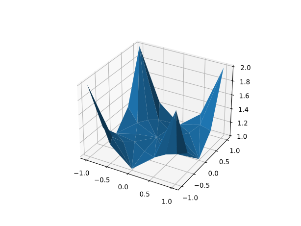
mgb_solution(m) returns the underlying classical solution object (the same MGBSOL that mgb_solve produces), so all of Plotting applies. Equivalently, value evaluates variables, deriv atoms, Coef data, and affine expressions of them as plain nodal vectors on geom, so anything in the nodal ordering plots directly:
plot(mgb_solution(m))                # component 1: u
plot(mgb_solution(m), 2)             # component 2: the slack s
plot(geom, value(u))                 # same picture as plot(mgb_solution(m))
plot(geom, value(deriv(u, :dx)))     # the derivative field ∂u/∂x
plot(geom, value(u - g))             # u minus the boundary data
This is exactly the package's default problem, so we can compare against the classical API on the same geometry. The lowering produces the identical discrete problem, so the solutions agree bit-for-bit:
sol_ref = mgb_solve(assemble(amg(geom); p = 1.5); verbose = false)
maximum(abs.(value(u) .- sol_ref.z[:, 1]))0.0The data model: nodal vectors, with sugar
Because the discretization is fixed when the model is built, every piece of spatial data — coefficients, Dirichlet values, starts, obstacle heights, variable exponents — boils down to a vector with one value per broken node. That vector is the fundamental form, and every data entry point accepts it directly:
Coef(m, vals::AbstractVector)set_start(u, vals::AbstractVector)EpiPower(pvals::AbstractVector)On(geom, mask::AbstractVector{Bool})— region membership, one Bool per node
Node i is vertex v of element e with i = v + (e-1)V where V = size(geom.x, 1): the rows of reshape(geom.x, :, d) are the node coordinates in this ordering, value returns solutions in it, and an On pair (v, e) selects entry v + (e-1)V. Functions and constants are syntactic sugar, resolved eagerly at modeling time: Coef(m, f) equals Coef(m, [f(x) at every node coordinate x]), and Coef(m, 0.5) equals Coef(m, fill(0.5, n)).
Next to a model variable, data needs no wrapper at all: u == g, u >= phi_vals, a * u, and w - image_vec resolve the Function or nodal vector through the adjacent operand's model, exactly as if wrapped in Coef. This gives Real vectors field semantics in the scalar algebra — u + v is one expression — while the broadcast u .+ v keeps its usual meaning (n elementwise expressions). In particular write @constraint(m, u >= vals), not u .>= vals: the broadcast form makes n copies of a global constraint, one per entry. Matrices are not data (nodal data is the flat length-V*N vector), and a Bool vector next to a variable is rejected as ambiguous — On(geom, mask) for a region, Coef(m, v) for genuine 0/1 data. The explicit Coef(m, ...) form remains for positions with no adjacent variable, such as a pure-data cone row built from a function.
xf = reshape(geom.x, :, 2)                       # broken-node coordinates
n  = size(xf, 1)
gv = [xf[i, 1]^2 + xf[i, 2]^2 for i in 1:n]      # nodal data, directly
value(Coef(m, gv)) == value(Coef(m, x -> x[1]^2 + x[2]^2))trueSince data goes in and solutions come out in the same nodal ordering, vectors round-trip: set_start(u, value(u)) warm-starts a model from a previous solve, and measured or precomputed nodal data (an image for ROF denoising, say) drops in directly, without wrapping it in an interpolating closure.
Regions: constraints on part of the domain
A constraint holds everywhere by default; adding On(...) restricts it to a node set of (vertex, element) pairs — the format of find_boundary and the low-level dirichlet_nodes API. On(geom, mask) is grid-level sugar for the same thing: a Bool mask over the nodal vectors (one entry per broken node, in the ordering of the data model), converted eagerly to the pair set. Equality + On is a Dirichlet condition; inequality/cone + On becomes a piecewise barrier, active only on the region. Region selection is ordinary data preparation — a comparison on the node coordinates gives the mask.
Here is a membrane pushed upward by a uniform load, with an obstacle imposed only on the left half of the domain:
geom2 = subdivide(fem2d_P2(), 3)
left = reshape(geom2.x, :, 2)[:, 1] .< 0     # Bool mask: nodes with x₁ < 0
phi = x -> 0.25 - x[1]^2 - x[2]^2            # the obstacle

m2 = MGBModel(geom2)
set_silent(m2)
@variable(m2, u2); @variable(m2, s2, Broken(), start = 100.0)
crBC  = @constraint(m2, u2 == 0.0, On(find_boundary(geom2)))
@constraint(m2, [deriv(u2, :dx); deriv(u2, :dy); s2] in EpiPower(2.0))
crObs = @constraint(m2, u2 >= phi, On(geom2, left))
@objective(m2, Min, integral(-1.0 * u2 + s2))
optimize!(m2)
plot(mgb_solution(m2))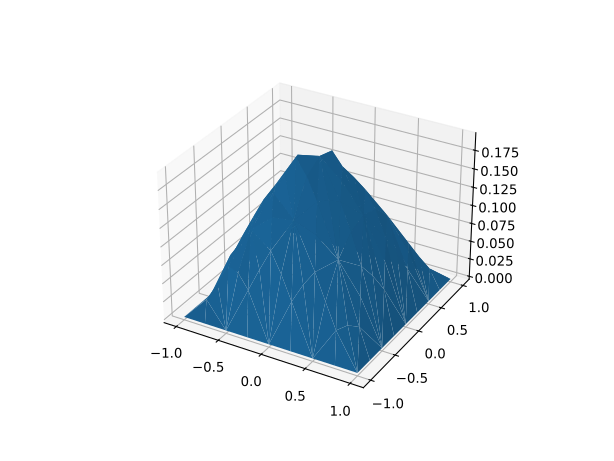
The obstacle binds on its region (the infeasible start is handled by the feasibility phase automatically) and is genuinely absent elsewhere — value evaluates the gap u - φ as an expression, and the mask indexes it directly:
gap = value(u2 - phi)
println("min(u - φ) on the obstacle region:  ", minimum(gap[left]))
println("min(u - φ) off the region:          ", minimum(gap[.!left]))
min(u - φ) on the obstacle region: 8.11009315260236e-11
min(u - φ) off the region: -0.05647391533765145Duals
After optimize!, dual(cr) returns the constraint's Lagrange multiplier as a nodal vector, in the same ordering as value. For inequality and cone constraints it is a density with respect to the volume measure — for the obstacle above, the contact pressure — read off the barrier gradient at the final barrier parameter, and accurate to O(tol) like the primal. It is zero off an On region, zero at nodes with zero quadrature weight (where the constraint is not collocated), nonnegative for >=, nonpositive for <= (the MOI convention; signs flip for Max, as in MOI). For EpiPower and SecondOrderCone rows, dual reports the multiplier of the pointwise epigraph inequality s ≥ ‖q‖ᵖ (not an MOI dual-cone vector).
One normalization rule to keep in mind: an inequality's dual is a density with respect to the volume measure, whether or not the constraint carries an On region. Its pointwise values are meaningful when the region has positive volume (an obstacle on a subdomain); on a lower-dimensional node set — a Signorini-type u >= 0, On(find_boundary(geom)) — the true multiplier is a boundary measure, and the volume-density values grow like the reciprocal mesh weight under refinement. Integrals remain correct in every case: sum(geom.w .* dual(cr) .* φ) is the pairing ⟨multiplier, φ⟩ regardless of the region's dimension. Equality duals (below) are the same object reported the other way — the multiplier's raw node masses, undivided — so their sums are the meaningful quantity.
pressure = dual(crObs)                       # contact pressure, one value per node
println("pressure off the region:       ", maximum(pressure[.!left]))
println("min pressure on the region:    ", minimum(pressure[left]))
println("complementarity ⟨pressure,gap⟩: ", sum(geom2.w .* pressure .* gap))
pressure off the region: 0.0
min pressure on the region: 2.562511983667302e-10
complementarity ⟨pressure,gap⟩: 3.5412864832573334e-9The dual of a Dirichlet equality is the reaction: the leftover objective gradient at the pinned coordinates (for a membrane, the boundary force holding the solution at g; discretely, the flux ∂u/∂ν). It is reported as raw per-broken-node forces — element shares, in the nodal ordering — not as a boundary density: an On set need not be a manifold, so no boundary measure is assumed. Coincident broken copies of a glued node sum to the physical nodal force, and the sum over the region is the total force:
reaction = dual(crBC)
println("total boundary reaction: ", sum(reaction))
total boundary reaction: -8.758241506172283The Zoo, restated in JuMP
Every Zoo problem is a few lines in this syntax; jump/test_zoo.jl checks all six against the classical constructors. Two examples. The minimal surface uses a constant row inside the cone — s ≥ ‖(∇u, 1)‖ is the shifted Lorentz cone (a plain 1.0 works; spatial data would be a Coef):
gu = x -> 0.5 * (x[1]^2 - x[2]^2)
ms = MGBModel(geom)
set_silent(ms)
@variable(ms, v, start = gu); @variable(ms, sv, Broken(), start = 10.0)
@constraint(ms, v == gu, On(find_boundary(geom)))
@constraint(ms, [deriv(v, :dx); deriv(v, :dy); 1.0; sv] in EpiPower(1.0))
@objective(ms, Min, integral(sv))
optimize!(ms)
ref = mgb_solve(Zoo.minimal_surface(amg(geom)); verbose = false)
maximum(abs.(value(v) .- ref.z[:, 1]))0.0Rudin–Osher–Fatemi denoising uses spatial data inside a cone — the fidelity slack is r ≥ (u - f_data)²:
fdata = x -> 0.5 * tanh(5 * x[1])
mr = MGBModel(geom)
set_silent(mr)
@variable(mr, w, start = fdata)
@variable(mr, sw, Broken(), start = 10.0); @variable(mr, r, Broken(), start = 10.0)
@constraint(mr, w == fdata, On(find_boundary(geom)))
@constraint(mr, [deriv(w, :dx); deriv(w, :dy); sw] in EpiPower(1.0))   # s ≥ |∇u|
@constraint(mr, [w - fdata; r] in EpiPower(2.0))                       # r ≥ (u-f)²
@objective(mr, Min, integral(sw + 0.5 * r))
optimize!(mr)
ref = mgb_solve(Zoo.rof(amg(geom)); verbose = false)
maximum(abs.(value(w) .- ref.z[:, 1]))0.0What lowers to what
| model content | classical object |
|---|---|
geometry passed to MGBModel | Geometry |
| variables, kinds, Dirichlet constraints | state_variables + dirichlet_nodes → amg(geom; dirichlet_nodes) |
distinct atoms (component, operator) used anywhere | the D table |
| each cone constraint | one Convex piece (convex_linear / convex_Euclidian_power); same-region scalar inequalities are merged into a single stacked piece |
On regions on cones | convex_piecewise selector columns |
integral(...) objective | the cost grid f_grid |
| starts + Dirichlet data | the initial/lift grid g_grid |
Untagged variables are conforming if differentiated or Dirichlet-constrained and broken otherwise; Broken() / Continuous() / Uniform() override. The notion of continuity is the geometry's connectivity geom.t, so slit domains built with explicit connectivity keep their slits. The model must be in conic form (epigraph slacks are yours to declare, as with any conic solver); pointwise equality requires On; @variable bounds and products of variable expressions are rejected with explanatory errors (spell bounds as pointwise constraints — the two-sided @constraint(m, lo <= u <= hi) works and lowers to two stacked inequalities). Spectral geometries work too, with one restriction inherited from their hierarchy: the spectral Dirichlet subspace is built by basis truncation, so a Dirichlet condition there must cover exactly the whole boundary (find_boundary(geom)). Constraint duals are available after the solve — see Duals.
Standard JuMP accessors
The usual JuMP workflow works unchanged: set_silent/unset_silent (they drive the "verbose" attribute), solution_summary, is_solved_and_feasible, termination_status (MOI.OPTIMAL on success — the problems are convex), objective_value, value (on variables, deriv atoms, Coef data, and affine expressions, always as a nodal vector), dual/has_duals/dual_status (see Duals), all_variables, start_value, has_values, raw_status, solve_time, and the result keyword (validated — there is exactly one result). @variable(m, u, start = data) accepts the same three data forms as set_start, and the integral objective is linear: 2*integral(u) - integral(s) equals integral(2*u - s). is_solved_and_feasible(m) is the recommended success check, and solution_summary(m; verbose = true) appends the solver iteration log (the same text as solver_log). JuMP's SecondOrderCone is accepted in its own epigraph-first convention: [s; q...] in SecondOrderCone() lowers identically to [q...; s] in EpiPower(1.0).
Three deliberate departures. Spatial data rides the scalar algebra: a Function or Real-eltype vector adjacent to a model variable is nodal data forming one field expression (u == g, u + v, phi_vals * u), where generic JuMP throws use-broadcasting errors for +/- and container-scales for *; broadcasting itself (u .+ v) keeps its usual elementwise meaning. Models are add-only: delete, fix, and the set_normalized_* modification API are not implemented — models are cheap, so rebuild instead (any structural mutation invalidates the previous result anyway). And the exported name MGBModel is the constructor function, not the model's type (the type lives in the extension because it must subtype JuMP.AbstractModel); annotate helper functions with f(m::JuMP.AbstractModel) if you need dispatch.
API reference
MultiGridBarrier.MGBModel — Function
MGBModel(geom::Geometry)Construct a JuMP model over a fixed MultiGridBarrier discretization. Requires using JuMP (which loads the modeling extension). Build it from any FEM or spectral Geometry (e.g. fem2d_P2(), subdivide(fem2d_P1(), 4), spectral2d(n = 16); spectral Dirichlet conditions must cover the whole boundary), then use the standard JuMP macros (@variable, @constraint, @objective); optimize! lowers the model to amg → assemble → mgb_solve, constructing the AMG hierarchy automatically from the geometry and the Dirichlet constraints. All spatial data (Coef) is per-broken-node vectors, resolved eagerly at modeling time (functions and constants are sugar for their nodal samples), and adjacent to a model variable both functions and nodal vectors appear directly in the algebra (u == g, phi_vals * u).
Solver options via set_attribute(m, key, value) with string keys "prolongator", "tol", "t", "t_feasibility", "feasibility_Rmax", "maxit", "kappa", "max_newton", "verbose", "device", "logfile"; unknown keys throw. JuMP's set_silent(m) / unset_silent(m) drive "verbose".
After optimize!, termination_status is MOI.OPTIMAL on success (the problems are convex, and the barrier method solves them to its tolerance); is_solved_and_feasible(m) is the standard check. Failures map the solver's diagnosis (MGBConvergenceFailure.code) to MOI: certified infeasibility is MOI.INFEASIBLE, exhausting the feasibility_Rmax bounding box is MOI.OTHER_LIMIT, a stalled t-ramp is MOI.SLOW_PROGRESS, hitting maxit is MOI.ITERATION_LIMIT, and anything else is MOI.OTHER_ERROR; raw_status carries the full diagnostic message in every case.
The concrete model type must subtype JuMP.AbstractModel, so it lives in the extension; the name exported here is the constructor function. For method signatures or isa checks, annotate with the JuMP abstract type — f(m::JuMP.AbstractModel) = ... — which is always in scope wherever a model can exist.
MultiGridBarrier.Coef — Function
Coef(m, v::AbstractVector{<:Real})
Coef(m, f::Function)
Coef(m, r::Real)
Spatial data for a MGBModel: one value per broken node. The nodal vector v is the fundamental form; it must have length V*N (V vertices per element, N elements), where entry i = v + (e-1)V belongs to vertex v of element e — the ordering of the rows of reshape(geom.x, :, d), of the vectors returned by value, and of the (v, e) pairs used by On. The other two forms are syntactic sugar, resolved eagerly on construction: Coef(m, f) is Coef(m, [f(x_i) for every node]), where f receives a node coordinate as a Vector and returns a Real, and Coef(m, r) is the constant vector Coef(m, fill(r, V*N)).
Adjacent to a model variable in expression algebra, data needs no wrapper: u == g, u >= phi_vals, a * u, and w - image_vec resolve the Function or nodal vector through the adjacent operand's model, exactly as if wrapped in Coef. (Real vectors get field semantics there — u + v is one expression — while broadcasting u .+ v keeps its usual elementwise meaning.) The explicit form remains for positions with no adjacent variable, such as a pure-data cone row built from a function.
MultiGridBarrier.deriv — Function
deriv(u, op::Symbol)The atom op applied to a model variable u, e.g. deriv(u, :dx). op must be a key of the geometry's operators (:id, :dx, :dy, ...). deriv(u, :id) is u.
MultiGridBarrier.integral — Function
integral(expr)The objective functional ∫ expr dx, where expr is affine in the model atoms; use inside @objective(m, Min, integral(...)). Integrals combine linearly — 2*integral(u) - integral(s) is integral(2*u - s) — but integral(u) + 3 is deliberately undefined (a bare constant has no ∫-form).
MultiGridBarrier.EpiPower — Function
EpiPower(p)The pointwise epigraph set { [q; s] : s ≥ ‖q‖₂^p }, used as @constraint(m, [q...; s] in EpiPower(p)) — slack LAST (the convex_Euclidian_power [q; s] convention). The exponent p ≥ 1 is spatial data in the same three forms as Coef: a per-node vector (the fundamental form), a spatial function x -> p(x), or a constant Real.
For p == 1, JuMP's SecondOrderCone is also accepted, in its own epigraph-first convention: @constraint(m, [s; q...] in SecondOrderCone()) lowers identically to [q...; s] in EpiPower(1.0).
MultiGridBarrier.On — Type
On(pairs::Vector{Tuple{Int,Int}})
On(geom::Geometry, mask::AbstractVector{Bool})
Constraint region for a MGBModel: a set of broken nodes as (vertex, element) pairs — the same format as find_boundary and the low-level dirichlet_nodes API. The second form is grid-level sugar: a Bool mask over the nodal vectors of Coef, converted eagerly to the pair set (mask[v + (e-1)V] selects vertex v of element e; the geometry supplies V). A mask composes directly with grid-level data: On(geom, reshape(geom.x, :, d)[:, 1] .< 0) is the left half of the domain. @constraint(m, u == g, On(pairs)) is a Dirichlet condition, where g is Coef data or a plain constant (u == 0.0); an inequality/cone with On holds only on those nodes.
MultiGridBarrier.Broken — Type
Broken()@variable tag for a MGBModel: the variable lives in the broken space (one degree of freedom per broken node) — the natural space for epigraph slacks. Untagged variables are broken by default when never differentiated or Dirichlet-constrained. See also Continuous.
MultiGridBarrier.Continuous — Type
Continuous()@variable tag for a MGBModel: the variable is a conforming (continuous) finite-element function, glued across elements. This is what untagged variables become when they are differentiated or Dirichlet-constrained; use the tag to force it for a variable that is neither — e.g. a slack you want continuous. (Note that constraining a slack to be continuous genuinely changes the optimum relative to Broken: the pointwise epigraph reformulation is exact only for broken slacks.)
The notion of continuity is the geometry's, not the tag's: DOFs are glued according to the connectivity geom.t. A slit/branch-cut domain built with an explicit connectivity (tensor_dofmap, the t= keyword of the mesh constructors, or gmsh_import's exact node tags) keeps coincident-but-distinct nodes separate, and Continuous() respects that gluing automatically — "continuous" then means continuous everywhere except across the slit.
MultiGridBarrier.Uniform — Type
Uniform()@variable tag for a MGBModel: the variable is a single global constant.
MultiGridBarrier.set_start — Function
set_start(u, v::AbstractVector{<:Real})
set_start(u, f::Function)
set_start(u, r::Real)
Initial iterate for component u of a MGBModel, as per-node data in the same three forms as Coef: a nodal vector (the fundamental form), or a spatial function / constant as sugar for it. value(u) returns solutions in the same nodal ordering, so set_start(u, value(u)) warm-starts from a previous solve. For Dirichlet-constrained variables the start doubles as the lift away from the constrained nodes; give slacks a comfortably feasible (large) start.
The @variable keyword accepts the same three forms (@variable(m, u, start = x -> ...)), and JuMP's start_value(u) reads the start back as a nodal vector (starts default to 0, so it never returns nothing).
MultiGridBarrier.mgb_solution — Function
mgb_solution(m::MGBModel) -> MGBSOLThe underlying MultiGridBarrier solution object after optimize! (for plot(sol), logs, etc.).
MultiGridBarrier.solver_log — Function
solver_log(m::MGBModel) -> StringThe MGB solver iteration log after optimize!.