API Guide

This page is the guided tour of the native (low-level) API: the workflow, the mesh constructors and their coordinate/connectivity conventions, and the hierarchy builders. For the high-level modeling front end see JuMP; for the docstrings see the API reference.

Workflow at a glance

Every problem is solved with the same four-step pattern:

1. Build a single-level Geometry with one of the mesh constructors (fem1d, fem2d, fem2d_P1, fem2d_P2, fem3d, spectral1d, spectral2d). These take only mesh inputs — no L, no hierarchy.
2. Attach a multigrid hierarchy with amg(geom) (algebraic multigrid). Returns a MultiGrid.
3. Assemble the problem with assemble(mg; kwargs...), returning an MGBProblem.
4. Solve with mgb_solve(prob; kwargs...).

To solve on a GPU, just load the CUDA extension (using CUDA, CUDSS_jll): with a functional GPU present, CUDADevice becomes the default device and every mgb_solve runs on the GPU with no code changes — the assembled problem is moved to the device, solved there, and the returned MGBSOL is moved back to native CPU types. Pass device = CPUDevice/CUDADevice to override per call; see CUDA.

If you want a finer mesh than the single-level geom provides, refine it first with subdivide(geom, L) and then attach AMG: amg(subdivide(geom, L)). The legacy geometric_mg(geom, L) builds a geometric-subdivision hierarchy instead of AMG; it is still available for callers that specifically want geometric transfers.

Choosing the AMG coarsening

For the FEM discretizations, amg(geom; prolongator=...) selects how the multigrid hierarchy is built. A prolongator is a callable mapping a stiffness matrix to its level prolongations; three factories are provided (each forwards keyword arguments such as max_coarse to the underlying builder):

• amg_ruge_stuben(; kwargs...) — classical Ruge–Stüben (the default), via AlgebraicMultigrid.jl.
• amg_smoothed_aggregation(; kwargs...) — smoothed aggregation, via the same package.
• amg_pyamg(; solver=:rootnode, kwargs...) — the Python pyamg package (:rootnode energy-minimization, :smoothed_aggregation, or :ruge_stuben); provided by the PyAMG extension (load PyCall).

mgb_solve(assemble(amg(fem2d_P1(); prolongator = amg_ruge_stuben(max_coarse=4)); p=1.5); verbose=false);

Finite elements

A 1d p-Laplace problem:

using MultiGridBarrier, PyPlot   # PyPlot enables the plotting extension
nodes = collect(range(-1.0, 1.0, length=33))
geom = fem1d(; nodes)
plot(mgb_solve(assemble(amg(geom); p=1.0); verbose=false));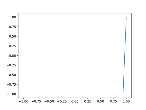

A 2d p-Laplace problem on tensor-product Q_k quadrilaterals (here biquadratic, k=2):

plot(mgb_solve(assemble(amg(subdivide(fem2d(; k=2), 3)); p=1.0); verbose=false));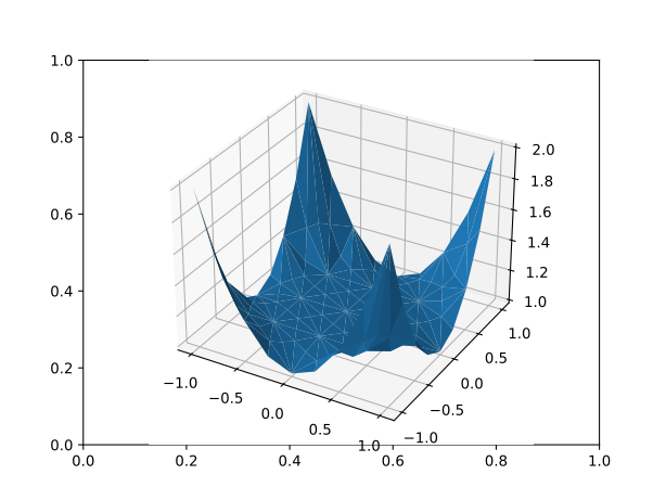

The same problem on P2+cubic-bubble triangles (fem2d_P2):

plot(mgb_solve(assemble(amg(subdivide(fem2d_P2(), 3)); p=1.0); verbose=false));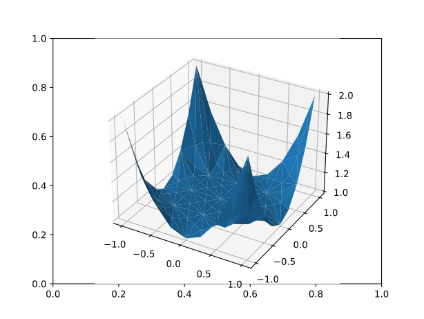

Spectral elements

1d p-Laplace via spectral elements:

plot(mgb_solve(assemble(amg(spectral1d(n=40)); p=1.0); verbose=false));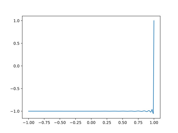

A 2d p-Laplace problem:

plot(mgb_solve(assemble(amg(spectral2d(n=5)); p=1.5); verbose=false));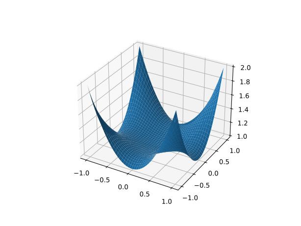

Solving $\infty$-Laplacians

For $p \geq 1$ on a domain $\Omega$, the $p$-Laplace problem minimises $J(u) = \|\nabla u\|_{L^p(\Omega)}^p + \int_{\Omega} fu,$ where $u$ lies in a suitable function space satisfying, e.g., Dirichlet conditions and $f$ is a forcing. The $\infty$-Laplace problem replaces the inner norm by $L^\infty$: $J(u) = \|\nabla u\|_{L^\infty(\Omega)}^p + \int_{\Omega} fu.$ We take $p=1$ below for simplicity.

plot(mgb_solve(assemble(amg(fem1d(; nodes)); p=1.0, state_variables=[:u :dirichlet; :s :uniform]); verbose=false));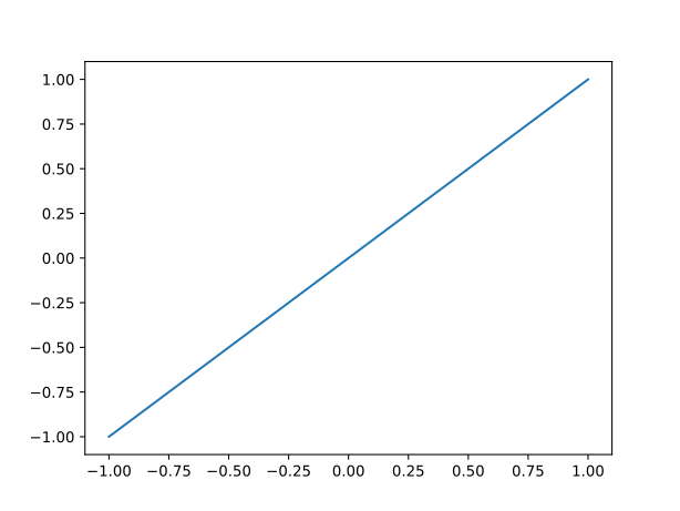

Parabolic problems

A time-dependent problem:

plot(parabolic_solve(amg(subdivide(fem2d_P1(), 3)); h=0.1, verbose=false))

3D Finite Elements

fem3d provides 3D hexahedral Q_k finite elements — the 3D case of the same dimension-generic tensor-product family as fem1d/fem2d — visualized with PyVista.

sol = mgb_solve(assemble(amg(subdivide(fem3d(; k=1), 2))); verbose=false)
fig = plot(sol)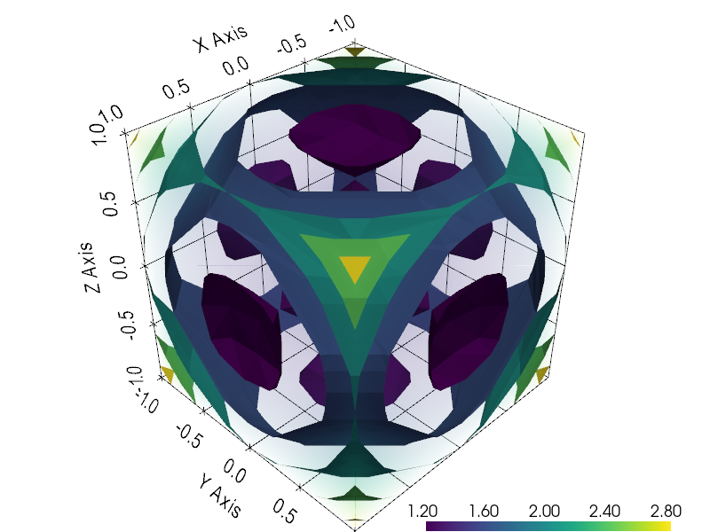

A time-dependent 3D problem:

plot(parabolic_solve(amg(subdivide(fem3d(; k=1), 2)); h=0.1, verbose=false))

Embedded manifolds

fem1d and fem2d also build embedded manifolds — a curve or surface living in a higher-dimensional ambient space — when you pass ambient=Val(e) together with a mesh K whose third dimension has e ≥ d coordinate columns. The cases are a curve in ℝ² or ℝ³ (fem1d, e = 2 or 3) and a surface in ℝ³ (fem2d, e = 3); the discretization type carries both dimensions as TensorFEM{d,e,T} (e.g. TensorFEM{2,3,Float64} is a surface in ℝ³).

On an embedded manifold the operators :dx, :dy[, :dz] are the e ambient components of the intrinsic (tangential) gradient ∇Γ — each output vector is tangent to the manifold, so `n · ∇Γ u = 0holds by construction and no normal vector is ever needed (which keeps higher codimension well-defined). The quadrature weightsgeom.ware the induced surface / arc-length measure√det(JᵀJ). Closed manifolds (circles, spheres, tori) close up automatically when coincident element corners are deduplicated; passt` explicitly for a glued/periodic mesh.

Everything downstream is unchanged: amg(geom), assemble, and mgb_solve work as usual. The only adjustment when posing a problem is that the operator matrix D must list all e ambient gradient components (e.g. :dx :dy :dz for a surface), since default_D keys on the intrinsic dimension; see test/test_manifold.jl for a worked scalar p-Laplace-plus-mass solve on a circle and a sphere.

Plotting follows one rule — graph the solution into the first free dimension, else show it as color: a curve in ℝ² is drawn as the height-graph (x, y, u), a curve in ℝ³ as a tube colored by u, and a surface in ℝ³ as a colored surface. For example, cos 2θ on the unit circle:

N = 120
θ = range(0, 2π, length=N+1)
K = zeros(2, N, 2)
for e in 1:N
    K[1, e, :] = [cos(θ[e]),   sin(θ[e])]
    K[2, e, :] = [cos(θ[e+1]), sin(θ[e+1])]
end
circle = fem1d(; K = K, ambient = Val(2))          # a curve in ℝ²: TensorFEM{1,2}
u = [cos(2 * atan(circle.x[v, e, 2], circle.x[v, e, 1]))
     for e in 1:size(circle.x, 2) for v in 1:size(circle.x, 1)]
fig = plot(circle, u)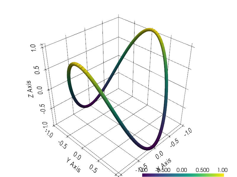

Front-end summary

The mesh constructors below all return a single-level Geometry. Boundary conditions are chosen later, at amg time, via its dirichlet_nodes keyword — the default constrains the whole boundary (homogeneous-trace Dirichlet); pass subsets or named node sets for mixed and per-component conditions.

fem1d/fem2d/fem3d are the tensor-product Q_k family (the map is isoparametric, so curved elements are supported); fem2d_P1/fem2d_P2 are the simplicial P_k family on triangles.

Every constructor except fem1d has a default mesh, and every other keyword is defaulted (including n for the spectral fronts); fem1d needs its element endpoints nodes — or the mesh tensor K passed directly. A mesh is fundamentally a connectivity/coordinates pair (t, x): you give the coordinates as K, and the tensor-product constructors fem1d/fem2d/fem3d take the connectivity as an optional t= keyword (deduced from the coordinates when omitted) — supply it for slit domains and glued manifolds where coincident nodes must stay distinct. See Meshes, coordinates, and connectivity.

Pass the resulting Geometry to amg(geom) to obtain a MultiGrid — an algebraic- multigrid hierarchy on the fine mesh. To refine the mesh first, compose with subdivide(geom, L): amg(subdivide(geom, L)).

The legacy geometric_mg(geom, L) builds a geometric-subdivision hierarchy instead of AMG; it remains available for callers that specifically want geometric transfers.

Visualization is an opt-in extension: load PyPlot (using MultiGridBarrier, PyPlot) and plot works on every solution and geometry — matplotlib for 1D/2D, PyVista for 3D volumes, surfaces, and curves; see Plotting. Without PyPlot the solver core has no Python dependency at all.

Prefer stating problems in an algebraic modeling language? The JuMP front end accepts standard @variable/@constraint/@objective syntax and lowers it to this same pipeline, building the hierarchy automatically.

Need meshes of real geometry (CAD shapes, holes, named boundary parts)? The Gmsh importer converts Gmsh meshes — P1/P2 triangles, and quads or hexahedra of any order, straight or curved — into a Geometry, and physical groups into named node sets for dirichlet_nodes and On.

Meshes, coordinates, and connectivity

Fundamentally a mesh — and the Geometry that holds it — is a pair (t, x):

• t, the connectivity (geom.t): an integer matrix of shape (V, N); t[v,e] is the global id of local node v in element e. It records which per-element nodes are the same global node, so maximum(geom.t) is the number of distinct nodes. The AMG hierarchy and find_boundary consult geom.t.
• x, the coordinates (geom.x): a 3-tensor of shape (V, N, D) in the broken / discontinuous-Galerkin layout — each element carries its own copy of every local node — giving the node positions (the geometry, possibly curved/isoparametric).

Keeping the two apart is the point: coincident nodes can be glued (one shared t id) or kept topologically distinct (different ids at the same coordinates). The latter — which no coordinate-only description can express — is how slit domains, branch cuts, and glued manifolds (e.g. the Riemann surface of √z) are represented. You pass the coordinates to the tensor-product constructors as the K keyword (it becomes geom.x) and the connectivity as the t keyword:

geom = fem2d(k = 2, K = coords, t = connectivity)

Convenience — omit t. For an ordinary embedded mesh you rarely have connectivity in hand, and you don't need it: leave t off and it is recovered automatically by deduplicating coincident coordinates (two per-element nodes at the same point become one global DOF). This is the everyday path — every example above uses it:

geom = fem2d(k = 2, K = coords)   # t deduced from coincident coordinates

Coordinates: the K tensor in detail

All FEM constructors take their coordinates as a K keyword argument (fem1d(; nodes) derives K from nodes by default). K is a 3-tensor K::Array{T,3} of shape (V, N, D):

• V is the number of local nodes per element. For the tensor-product Q_k family it is (k+1)^d: k+1 for fem1d, (k+1)^2 for fem2d, (k+1)^3 for fem3d (you may instead pass the 2^d-corner tensor — 2, 4 or 8 — for straight elements, which is promoted internally). For the simplicial family V is 3 for fem2d_P1, and 7 for fem2d_P2 (6 with bubble=false);
• N is the number of elements;
• D is the ambient (embedding) dimension — the number of coordinate components, 1, 2, or 3. For an ordinary codimension-0 mesh it equals the intrinsic element dimension d (1 for fem1d, 2 for fem2d, 3 for fem3d); for an embedded manifold (a curve or surface living in a higher-dimensional space) it exceeds d — see Embedded manifolds below.

K[v, e, d] is the d-th coordinate of the v-th local node of the e-th element. So in 1D, nodes x[1] < x[2] < … < x[m] defining elements [x[1],x[2]], [x[2],x[3]], …, [x[m-1],x[m]] give a (2, m-1, 1) tensor

K = reshape(T[x[1], x[2], x[2], x[3], x[3], x[4], …, x[m-1], x[m]], 2, m-1, 1)

with each interior node appearing twice (once per neighbouring element). The stored geom.x carries the same shape as K; the flat (V·N, D) view used by sparse operators is recovered via reshape(geom.x, :, size(geom.x, 3)).

Spectral discretizations (spectral1d, spectral2d) have no element structure and use N = 1 — geom.x has shape (n, 1, 1) in 1D and (n², 1, 2) in 2D.

Building t for high order: tensor_dofmap

A mesh generator gives you corner connectivity (2^d × N), but a Q_k mesh also needs a global id for every edge/face/interior node. tensor_dofmap builds the full (k+1)^d × N connectivity from corner connectivity t_corner alone — no coordinates — numbering shared edges/faces consistently (with edge orientation at k≥3), so any slit/branch-cut structure in the corner connectivity propagates to the high-order nodes. It supports any d for k≤2 and any k for d≤2; it throws on shared 3D face-interior grids (d≥3, k≥3), where you supply t by hand or use the dedup default.

For example, two Q2 quads sharing the seam x = 1:

# coordinates (corner shorthand): [0,1]² and [1,2]×[0,1]
K = reshape(Float64[0 0; 1 0; 0 1; 1 1;        # element 1 corners
                    1 0; 2 0; 1 1; 2 1],       # element 2 corners
            4, 2, 2)

glued = fem2d(k = 2, K = K, t = tensor_dofmap([1 2; 2 5; 3 4; 4 6], 2, Val(2)))  # 15 nodes
slit  = fem2d(k = 2, K = K, t = tensor_dofmap([1 7; 2 5; 3 8; 4 6], 2, Val(2)))  # 18 nodes

The coordinates are identical; only the connectivity differs. In glued the seam is a shared interior edge (15 distinct nodes); in slit element 2's left corners carry distinct ids 7, 8, so the seam splits into two boundaries (18 distinct nodes) — a result the coordinate-dedup default cannot produce.

amg vs subdivide vs geometric_mg

• amg(geom) is the recommended hierarchy: it builds AMG from the fine mesh's continuous-P1 stiffness. Works whether geom came from your own mesher or from uniform subdivision via subdivide.
• subdivide(geom, L) is mesh refinement only: it returns a fine Geometry obtained by subdividing each input element L−1 times. Compose with amg(subdivide(geom, L)) to get AMG on the refined mesh.
• geometric_mg(geom, L) is the legacy alternative: it produces a hierarchy of L levels using purely geometric subdivision transfers (no AMG coarsening). Kept for cases that need geometric transfers specifically.

Reference

The full docstring reference (module, types, functions, and the index of all documented names) lives on the API reference page; the extension APIs are documented on the Plotting, JuMP, Gmsh, and PyAMG pages.